

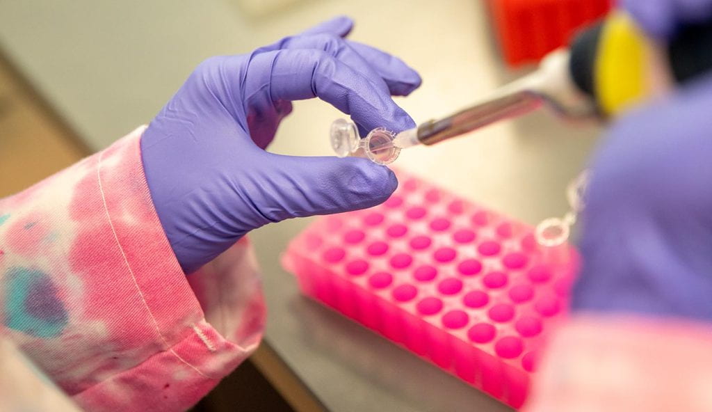
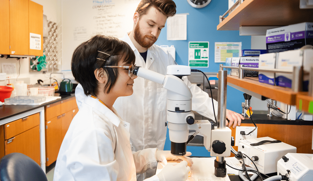
The Biomolecular Engineering (BME) Department within the Baskin School of Engineering features an interdisciplinary blend of engineering, biology, chemistry, and statistics designed to foster collaboration with other departments. This blend reflects our vision of the direction that biomedical discovery will take over the next two decades.
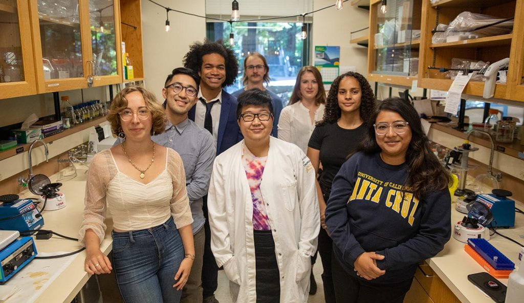
Members of the Biomolecular Engineering Department collaborate actively with faculty from other engineering departments and with the Physical and Biological Sciences departments of Molecular, Cell, and Developmental Biology, Chemistry and Biochemistry, Microbiology and Environmental Toxicology, Ecology and Evolutionary Biology, and Ocean Sciences.

1st
to complete a gapless sequence of a human genome
#2
public university in the nation for students focused on making an impact in the world (Princeton Review, 2022)
AAU
in 2019, UCSC was named to the Association of American Universities, joining just 65 other universities
Solving a centuries-old origins of animal life mystery

Researchers discovered the pivotal moment when the comb jelly, an ancient organism, became the first to diverge from the animal tree of life—providing new insight into how key features of animal anatomy have evolved over time.
BME Research News
Career Opportunities with a Biomolecular Engineering Degree

- Research Scientist
- Product Manager
- Engineer
- Field Technician
- Process Engineer
- IT Specialist/Analyst